Misc

Plotting spectral sequences

I spend a lot of time computing spectral sequences, and the various software available to plot spectral sequences is indispensable. I use Bruner’s ext software constantly to compute $Ext_{\mathcal{A}}$ and $Ext_{\mathcal{A}(2)}$ and plot the corresponding Adams charts. I use Hood Chatham’s spectral sequences package to display spectral sequences in Latex documents.

In a different direction, my brother Darius Carrick and I are working on a React app ssplot to plot bigraded rings from Macaulay2 output onto a grid using Google charts. This works pretty well if you are just trying to explore a spectral sequence page-by-page without plotting differentials, structure lines, etc., though we plan to add this functionality as well. It works especially well if you are working with trigraded SS’s and you want to plot some bigraded plane. For instance, with slice SS’s it is easier to describe the pages as $RO(G)$-graded rings, but you would like a plot of the SS in integer stems.

Example: Adams spectral sequence for $ko$

As an example, let’s plot the $E_2$ page of the ASS for $ko$. Here we have

\[Ext_{\mathcal{A}_*}(\mathbb{F}_2,H_*ko)\cong Ext_{\mathcal{A}(1)_*}(\mathbb{F}_2,\mathbb{F}_2)\cong\mathbb{F}_2[h_0,h_1,b,B]/(h_0h_1,h_1^3,h_1b,b^2-h_0^2B)\]

The generators have the following Adams bidegrees

\[\begin{align*} |h_0|&=(0,1)\\ |h_1|&=(1,1)\\ |b|&=(4,3)\\ |B|&=(8,4) \end{align*}\]

We can define this ring in Macaulay2 as follows.

R = ZZ/2[h0,h1,b,B,Degrees=>{{0,1},{1,1},{4,3},{8,4}}]/ideal{h0*h1,h1^3,h1*b,b^2-h_0^2*B}

You can ask Macaulay2 for a basis of any given bidegree, and the following gives us a basis of bidegrees $(t-s,s)=(x,y)$ for $0\le x,y\le 50$.

for i from 0 to 50 list (for j from 0 to 50 list (i,j,toString flatten entries basis({i,j},R),length flatten entries basis({i,j},R)))

Here’s how this looks in the Macaulay2 web terminal available here:

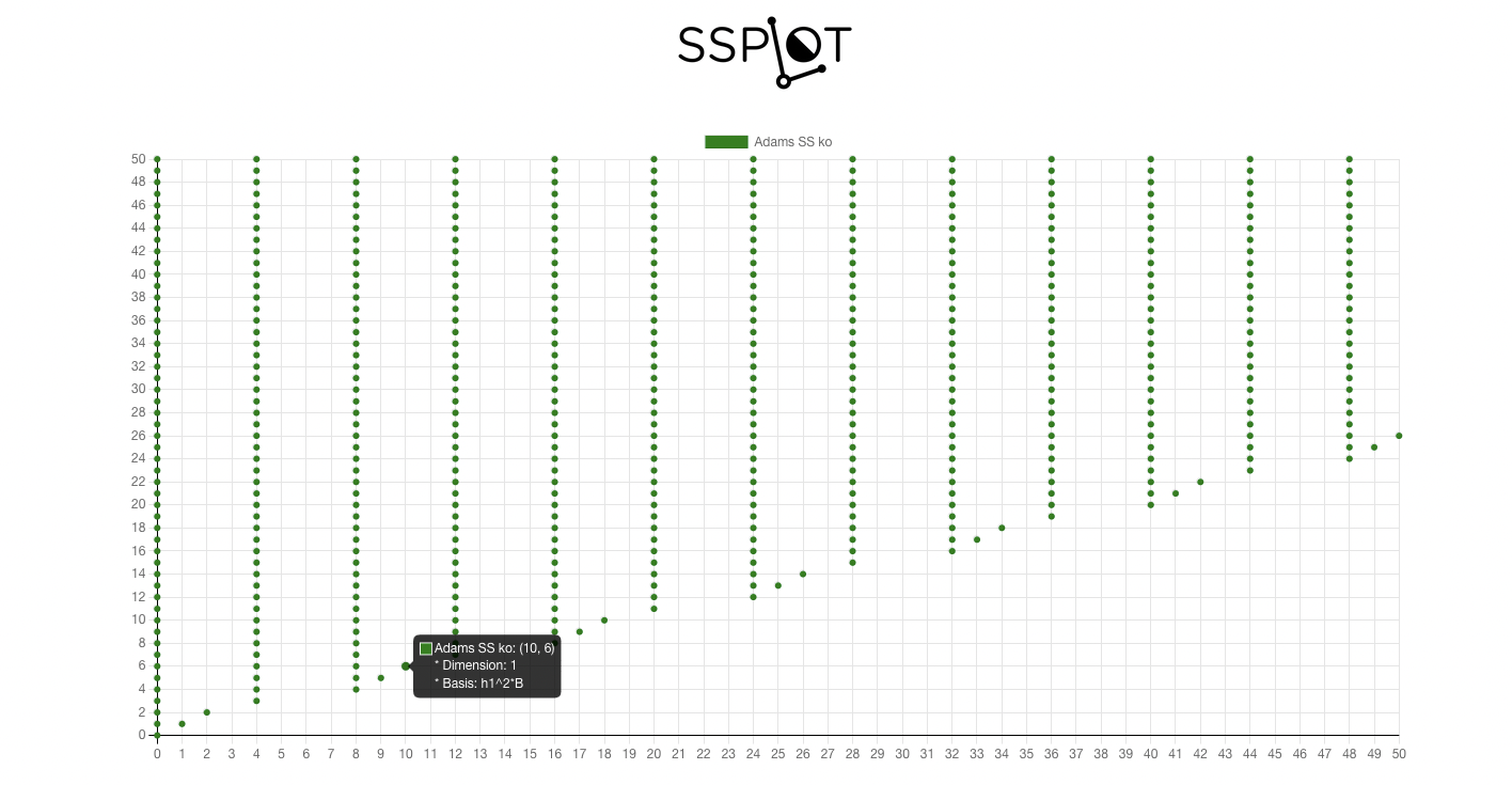
Copying the text from the line o2 and pasting into ssplot, we have the following:

Hovering over a dot gives the dimension and basis for that bidegree.

Example: Slice$(k_\mathbb{R})$

As a slightly more complicated example, let’s plot the (integer-graded, i.e. bidegrees $(a+b\sigma,s)$ with $b=0$) pages of the slice spectral sequence for $k_{\mathbb{R}}=BP_{\mathbb{R}}\langle 1\rangle$. It has $RO(C_2)$-graded $E_2$-page

\[E_2=\mathbb{Z}[a_\sigma,u_{2\sigma},\overline{v}_1]/(2a_\sigma)\]

The generators have the following bidegrees

\[\begin{align*} |a_\sigma|&=(-\sigma,1)\\ |u_{2\sigma}|&=(2-2\sigma,0)\\ |\overline{v}_1|&=(1+\sigma,0) \end{align*}\]

We can define this ring in Macaulay2 (as a trigraded ring $(a,b,s)$ corresponding to stem $a+b\sigma$ in filtration $s$) as follows.

E2 = ZZ[a,u,v,Degrees=>{{0,-1,1},{2,-2,0},{1,1,0}}]/ideal{2*a}

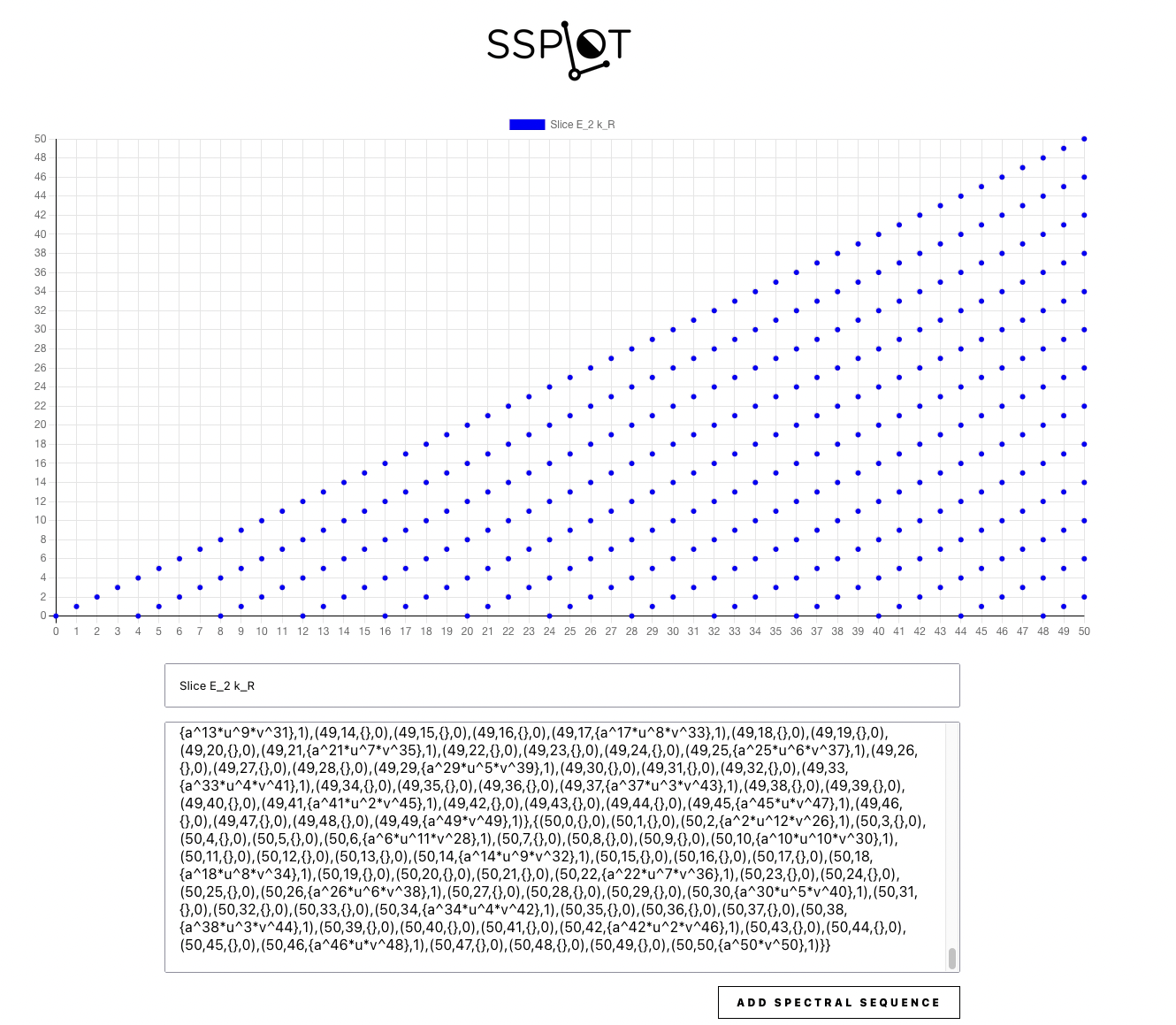
This time we need to change the code to make sure we only get classes in weight 0 (although we could do the same to get the bigraded page for any fixed weight). Here $j$ goes from $0$ to $i$ because the $C_2$-slice SS for a slice connective theory always lies between $y=0$ and $y=x$.

for i from 0 to 50 list (for j from 0 to i list (i,j,toString flatten entries basis({i,0,j},E2),length flatten entries basis({i,0,j},E2)))

This outputs the following.

This spectral sequence has just one differential, $d_3(u_{2\sigma})=a_\sigma^3\overline{v}_1$. Computing homology, we have

\[E_4=\mathbb{Z}[a_\sigma,m_1,u_{2\sigma}^2,\overline{v}_1]/(2a_\sigma,a_\sigma m_1,m_1^2-4u_{2\sigma}^2,a_\sigma^3\overline{v}_1)\]

where $m_1=[2u_{2\sigma}]$. All the algebra generators now are permanent cycles, so this is the $E_\infty$-page. We input this into Macaulay2 as follows

Einfty = ZZ[a,m,u,v,Degrees=>{{0,-1,1},{2,-2,0},{4,-4,0},{1,1,0}}]/ideal{2*a,a*m,m^2-4*u,a^3*v}

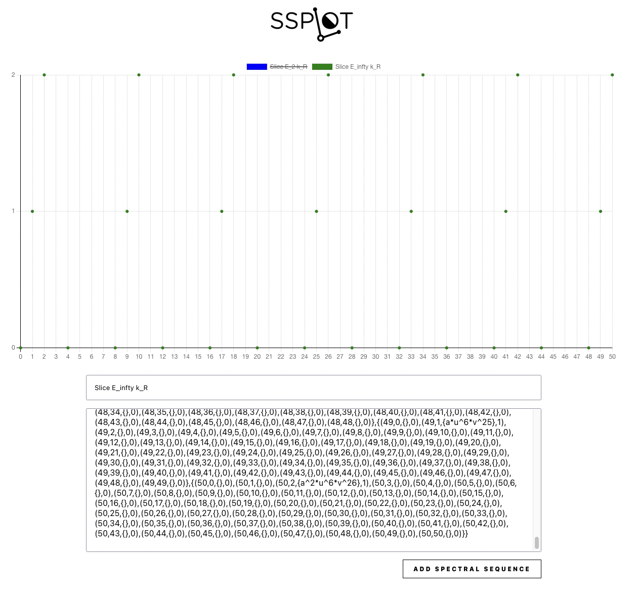
Getting a basis through the 50 stem and plugging into ssplot we have the following picture of $E_\infty$.

Here’s how this all looks in the Macaulay2 terminal:

We see the expected 8-fold Bott periodicity. By clicking the bars at the top, we can toggle the pages or display them simultaneously.